
Diffusion Equation
Published:
\begin{align} \frac{\partial u}{\partial t} = \alpha \frac{\partial^2 u}{\partial x^2}, \quad \quad x \in (-L/2,L/2), \quad t \in (0,T] \tag{1} \end{align}
with initial condiditon
\[u(x,0) = f(x)\]and boundary coundition
\[u(-L/2) = 0 \quad \text{and} \quad u(L/2) = 0\]Since Eq. 1 is a linear partial differential equation we can consider the solution of the equation in the fourier space.
Let the solution in the fourier space be $\hat{u}(k,t)$, where $k$ represents the $k^{th}$ mode of the solution in the fourier space. Therefore for any mode $k$, the solution in the real space will be $\hat{u}e^{ikx}$ and it should satisfy Eq. 1. (Integration over k will give the complete solution)
\[\begin{aligned} \frac{d \hat{u}}{d t}e^{ikx} &= \alpha (ik)^2 e^{ikx}\hat{u} \\ \frac{d \hat{u}}{d t} &= -\alpha k^2 \hat{u} \\ \hat{u}(k,t) &= \hat{u}(k,0)e^{-\alpha k^2 t} \\ \end{aligned}\]Therefore the solution in our real space for the $k^{th}$ mode will be
\[u(x,t) = \hat{u}(k,0)e^{ikx}e^{-\alpha k^2 t} \tag{2}\]Eq. 2 shows that the amplitude of each of $k^{th}$ mode decreases exponential with the rate $\alpha k^2$. This means the high frequency modes damp out faster that the low frequency modes.
Discretisation
Spatial variable \(x_i = -L/2 + i \Delta x \quad i=0,...,N_x\) where $ L = \Delta x N_x $
Temporal variable \(t_n = n \Delta t \quad n=0,...,N_t\) where $ T = \Delta t N_t $
With $u^{n}_{i}$ denoting the approximate solution for $u(t_n,x_i)$.
Forward Euler Explicit Scheme
Finite Difference Approximation
Forward difference in time and central difference in space
\[\frac{u_{i}^{n+1}-u_{i}^{n}}{\Delta t} = \alpha \frac{ u_{i+1}^{n} - 2u_{i}^{n} + u_{i-1}^{n} }{\Delta x^2}\]Hence we derived an approximation for Eq. 1 which is completely algebric and the unknown variable $u_{i}^{n+1}$ is a function of all the known variables.
\(u_{i}^{n+1} = u_{i}^{n} + F(u_{i+1}^{n} -2 u_{i}^{n} + u_{i-1}^{n})\) for $i=1,…,N_x-1$
(Note for $i=0$ and $i=N_x$ we have the boundary conditions)
Here $F = \alpha \Delta t / \Delta x^2$ is a dimensionless number in the equation which takes into account all the key parameters in the discretised problem. All the properties of the numerical method are critically dependent upon the value of $F$.
from numpy import *
import matplotlib.pyplot as plt
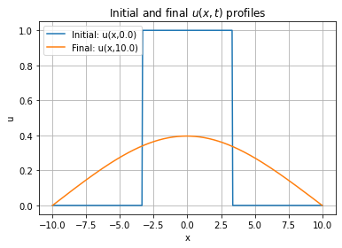
def initialCondition(x):
N = len(x)
u = zeros(N)
#u = e**(-x**2)
u[int(N/3.0):int(2.0*N/3.0)] = 1.0
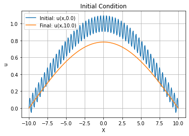
#u = cos(x*pi/x[-1]/2.0) + 0.1*cos(101.0*x*pi/x[-1]/2.0)
plt.plot(x,u, label='Initial: u(x,0.0)')
plt.title(r"Initial and final $u(x,t)$ profiles")
plt.xlabel("x")
plt.ylabel("u")
return u
L = 20.0
T = 10.0
a = 1.0

Nx = 401
Nt = 8100

x = linspace(-L/2, L/2, Nx+1)    # mesh points in space
dx = x[1] - x[0]
t = linspace(0, T, Nt+1)    # mesh points in time
dt = t[1] - t[0]
F = a*dt/dx**2

print(f'The value of F if {F}')

u = zeros(Nx+1)
uOld = zeros(Nx+1)
uOld = initialCondition(x)

# Time Stepping
for n in range(Nt):

  # Boundary Condiditons
  u[0] = 0; u[Nx] = 0;

  # Computing u at inner mesh points
  for i in range(1,Nx):
    u[i] = uOld[i] + F*(uOld[i+1] - 2*uOld[i] + uOld[i-1])

  # Updating u
  uOld = u

plt.plot(x,u,label=f'Final: u(x,{T})')
plt.legend(loc="upper left")
plt.grid(True)
plt.show()
The value of F if 0.496299382716067
Results
Backward Euler Implicit Scheme
Finite Difference Approximation
Backward difference in time and central difference in space
\[\frac{u_{i}^{n}-u_{i}^{n-1}}{\Delta t} = \alpha \frac{ u_{i+1}^{n} - 2u_{i}^{n} + u_{i-1}^{n} }{\Delta x^2}\]Hence we derived an approximation for Eq. 1 which is a $(N_x-1) \times (N_x-1)$ system of linear equations
\(-Fu_{i+1}^{n} +(1 + 2F) u_{i}^{n} -Fu_{i-1}^{n} = u_{i}^{n-1}\) for $i=1,…,N_x-1$
(Note for $i=0$ and $i=N_x$ we have the boundary conditions).
The above system can be numerically solved by
- Gauss elimination
or iterative methods like
- Jacobi
- Gauss Seidel
- Multigrid
These iterative methods are explained in [make a jupyter notebook]. For now we will use the the linear system solver that comes in numpy.linalg
L = 20.0
T = 10.0
a = 1.0

Nx = 401
Nt = 2100

x = linspace(-L/2, L/2, Nx+1)    # mesh points in space
dx = x[1] - x[0]
t = linspace(0, T, Nt+1)    # mesh points in time
dt = t[1] - t[0]
F = a*dt/dx**2

print(f'The value of F if {F}')

u = zeros(Nx+1)
uOld = zeros(Nx+1)
uOld = initialCondition(x)

A = zeros((Nx+1,Nx+1))
b = zeros((Nx+1,))

# Boundary Condition (A matrix does not change with time)
A[0,0] = 1.0
A[Nx,Nx] = 1.0
b[0] = 0.0
b[Nx] = 0.0

# Time Stepping
for n in range(Nt):

  # Making the linear system
  for i in range(1,Nx):
    A[i,i] = 1.0 + 2.0*F
    A[i,i+1] = -F
    A[i,i-1] = -F
    b[i] = uOld[i]

  # Solving the linear system
  u = linalg.solve(A,b)

  # Updating u
  uOld = u

plt.plot(x,u,label=f'Final: u(x,{T})')
plt.legend(loc="upper left")
plt.grid(True)
plt.show()
The value of F if 1.914297619047687
Stability Analysis
As seen earlier, any solution to Eq. 1 can be written as linear combination of different modes where any $k^{th}$ mode evolves as $ u(x,t) = \hat{u}(k,0)e^{ikx}e^{-\alpha k^2 t} $ and its amplitude is determined by the initial condition.
Since all these modes are linearly independent we can consider any particular mode for our analysis.
Let our initial condition be \(u(x,0) = e^{ikx}\) which after $\Delta t$ time becomes \(u(x,\Delta t) = e^{-\alpha k^2 \Delta t} e^{ikx}\) thus we get an actual amplification \(A_e = e^{-\alpha k^2 \Delta t}\)
Forward Euler
In case of forward euler we get an amplification of \(A = 1 - 4F Sin^2\bigg( \frac{k \Delta x}{2} \bigg)\) For the scheme to be stable$ |A| \leq 1 $ , which gives us \(F \leq \frac{1}{2}\)
Backward Euler
In case of backward euler we get an amplification of \(\frac{1}{A} = 1 + 4F Sin^2\bigg( \frac{k \Delta x}{2} \bigg)\) For the scheme to be stable $ |A| \leq 1 $ , which is always true in this case.
Hence backward euler scheme is unconditionally stable.