Mechanochemical Pattern Formation
Published:
Actomyosin Cortex
The actomyosin cortex of a cell is composed of actin filaments and myosin motor proteins.
Actin Filaments
The actin filaments exits in two forms- as polymeric form beneath the cell membrane and as monomeric form in the cytosol. The filament polymerises and depolymerises releasing any elastic stress in the cortex. Thus we can write a hydrodynamic description of the cortex at time scales larger than this turn over time scale.
Myosin Motors
The myosin motors consume ATP and generate contractile forces in the cortex. Thus a gradient in the concentration of these myosin motors lead to a gradient in the contractile tension in the cortex. This gradient results in a flow field.
Active hydrodynamic theory of actomyosin cortex
Since there is a constant influx of energy, as myosin motors consume ATP to generate contractile forces, we call this system active.
Consider an active stress regulator chemical whose concentration is given by $c$
\[\frac{\partial c}{\partial t} = \frac{\partial ^2 c}{\partial x^2} -Pe \frac{\partial vc}{\partial x}\]The chemical species is advected by the flow field generated due to the active stress and the chemical species itself is responsible for generating the active stress. Thus there is a coupling between the chemical species and the underlying mechanics of the cortex.
The force balance equation for the active fluid (neglecting the inertial forces and assuming that the flow field relaxes instantly)
\[\partial_x\sigma - \gamma v = 0\]where $\gamma$ is the friction coefficient from the surrounding medium and $\sigma = \sigma_{viscous} + \sigma_{active}$ and the active stress is some function of $c$
The nondimensionalized form becomes
\[\frac{\partial^2 v}{\partial x^2} + \frac{\partial }{\partial x} f(c) = v\]where $f(c) = \big(\frac{c}{1+c}\big)$
Perturbing the system about the steady state $(c_0,0)$
\[c = c_0 + \delta c = c_0 + \delta c_0 e^{ikx}\]The perturbation in $c$ generates a flow field given by
\[v = \frac{\delta c (ik) \partial_c f}{1+k^2}\]Putting the flow field back into the $c$ evolution equation to check the stability of $k^{th}$ mode (linear order).
\[\frac{\partial \delta c_0}{\partial t} = -k^2 \delta c_0 \bigg(1-\frac{Pe c_0 \partial_cf}{1+k^2}\bigg)\]Hence we get the condition for instability
\[\frac{Pe c_0 \partial_cf}{1+k^2} > 1\]from numpy import *
from numpy import random
import matplotlib.pyplot as plt
%matplotlib inline
from IPython import display
L = 3*pi
T = 10.0

mode = 6.
c0 = 1.

Pe = 42.

Nx = 101
Nt = 50000

x = linspace(0., L, Nx+1)    # mesh points in space
dx = x[1] - x[0]
t = linspace(0, T, Nt+1)     # mesh points in time
dt = t[1] - t[0]

print(f'The value of F if {dt/dx**2}. It should be less that 0.1 for numerical stability.')

# f(c)=c/(1+c); df/dc=1/(1+c)^2
dfdc_c0 = 1.0/(1.0 + c0)**2
instability = Pe*c0*dfdc_c0/(1. + mode**2)
print(f'For instability {instability} should be greater than 1')
The value of F if 0.022968386540788612. It should be less that 0.1 for numerical stability.
For instability 0.28378378378378377 should be greater than 1
def ReactionDiffusionNeumannII(c, t, dx, v):

    N = len(c)
    # Central difference for interior and Periodic BC for right and left boundary
    Diffusion = array([c[i+1] - 2*c[i] + c[i-1] for i in r_[1:N-1]])
    # Left boundary condition
    Diffusion_L = c[1] - 2*c[0] + c[0]
    # Right boundary condition
    Diffusion_R = c[-1] - 2*c[-1] + c[-2]
    Diffusion = r_[Diffusion_L,Diffusion,Diffusion_R]/dx**2


    Advection = array([v[i+1]*c[i+1] - v[i-1]*c[i-1] for i in r_[1:N-1]])
    Advection_L = v[1]*c[1] - v[-2]*c[-2]
    Advection_R = v[1]*c[1] - v[-2]*c[-2]
    Advection = r_[Advection_L,Advection,Advection_R]/2/dx

    return Diffusion - Pe*Advection
def RK4_timestepper(fun,y0,dt,args):

    y = y0

    k1 = fun(y,t,*args)
    k2 = fun(y+0.5*dt*k1,t+0.5*dt,*args)
    k3 = fun(y+0.5*dt*k2,t+0.5*dt,*args)
    k4 = fun(y+dt*k3,t+dt,*args)

    y = y + (k1 + 2*k2 + 2*k3 + k4)/6.*dt

    return y
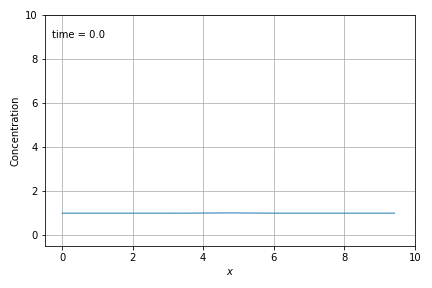
def initialCondition(x):
N = len(x)
c = zeros(N)
# c = c0 + 0.01*random.rand(N)
# c = c0 + cos(mode*x*pi/3./pi)
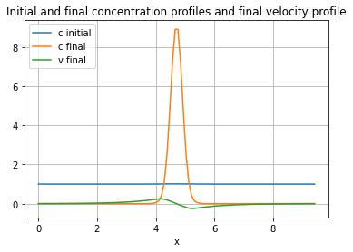
c = c0 + 0.01*exp(-mode*(x-L/2)**2*pi/3./pi)
plt.plot(x,c,label='c initial')
plt.title(r"Initial and final concentration profiles and final velocity profile")
plt.xlabel("x")
return c
c = zeros(Nx+1)
v = zeros(Nx+1)
cOld = zeros(Nx+1)
cIni = zeros(Nx+1)
cIni = initialCondition(x)
cOld = cIni
A = zeros((Nx+1,Nx+1))
b = zeros((Nx+1,))
# Boundary Conditions for velocity
A[0,0] = 1.0
A[Nx,Nx] = 1.0
b[0] = 0.0
b[Nx] = 0.0
Time = [t[0],]
Conc = [cIni,]
Velo = [v,]
# fig, (ax1, ax2) = plt.subplots(nrows=2, figsize=(8,8))
# Time Stepping
for n in range(Nt):
# Boundary Condiditons
# cOld[0] = cOld[Nx-1]; cOld[Nx] = cOld[1]; # Periodic BC
cOld[0] = cOld[1]; cOld[Nx] = cOld[Nx-1]; # No Flux BC
# plt.plot(x,cIni,label='Initial t=0')
# plt.plot(x,cOld,label='Profile at t=%0.3lf'%(n*dt))
# plt.legend(loc="upper left")
# display.display(plt.gcf())
# display.clear_output(wait=True)
# Solving for the steady state velocity profile
# Making the linear system
for i in range(1,Nx):
A[i,i] = - 1.0 - 2.0/dx/dx
A[i,i+1] = 1/dx/dx
A[i,i-1] = 1/dx/dx
b[i] = -(cOld[i+1]-cOld[i-1])/2/dx/(1+cOld[i])**2
# Solving the velocity linear system
v = linalg.solve(A,b)
c = RK4_timestepper(ReactionDiffusionNeumannII,cOld,dt,(dx,v))
if (n+1)%500==0:
Time.append((n+1)*dt)
Conc.append(c)
Velo.append(v)
# Updating u
cOld = c
plt.plot(x,c,label='c final')
plt.plot(x,v,label='v final')
plt.legend(loc="upper left")
plt.grid(True)
plt.show()